Analyzer
Once the Processor has finished processing all interferograms, the Analyzer panel runs time-series analysis on the resulting products.
Initializing the Analyzer
Once all submitted jobs have finished and show SUCCEEDED in the Processor panel, open the Run Analyzer tab within the same job folder. Select an analyzer type (e.g. Hyp3_Mintpy_SBAS) from the drop-down and click Init to initialize the analyzer workspace. This prepares the configuration and directory structure needed to run time-series analysis on the downloaded interferograms. Different analyzer might have different steps.
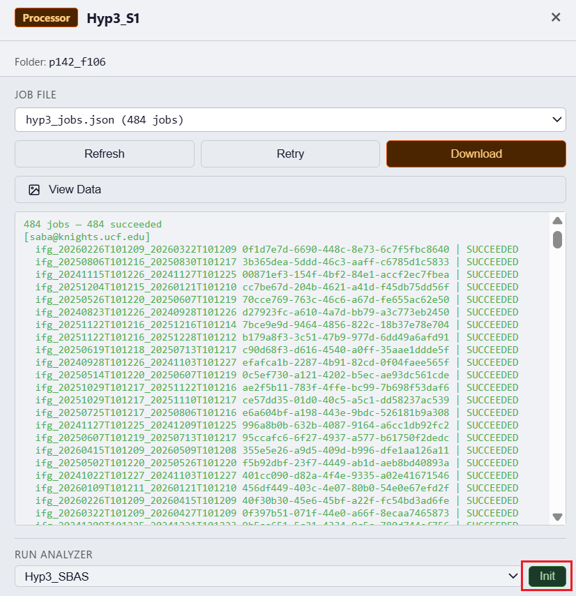
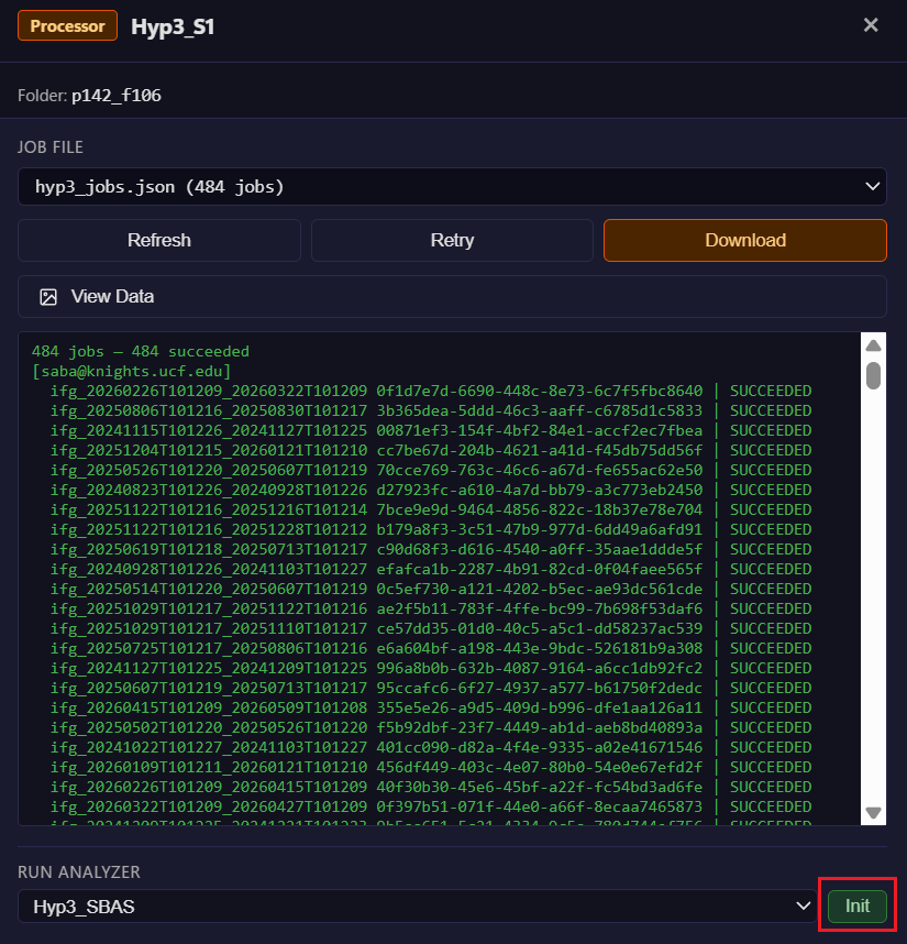
The Run Analyzer tab — select an analyzer type and click Init to get started.
Once initialization is complete, an Analyzer tag labeled with the analyzer you chose (e.g. Hyp3_Mintpy_SBAS) will appear on the job folder. Click that tag to open the Analyzer panel and proceed with configuration and processing.
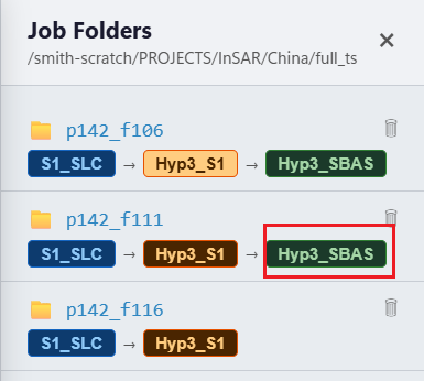
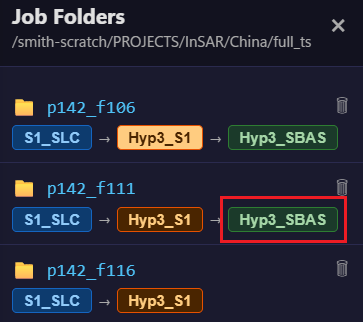
The Analyzer tag appears on the job folder after initialization. Click it to open the Analyzer panel.
Configuration
Once you enter the Analyzer panel, you can select the steps you want to run for time-series analysis. To adjust analysis parameters, click Change Config to switch to the configuration tab, where each analyzer type (e.g. Hyp3_Mintpy_SBAS) has its own independent settings that are saved separately.
For a full description of all analyzer parameters and options, see the Analyzer Reference.
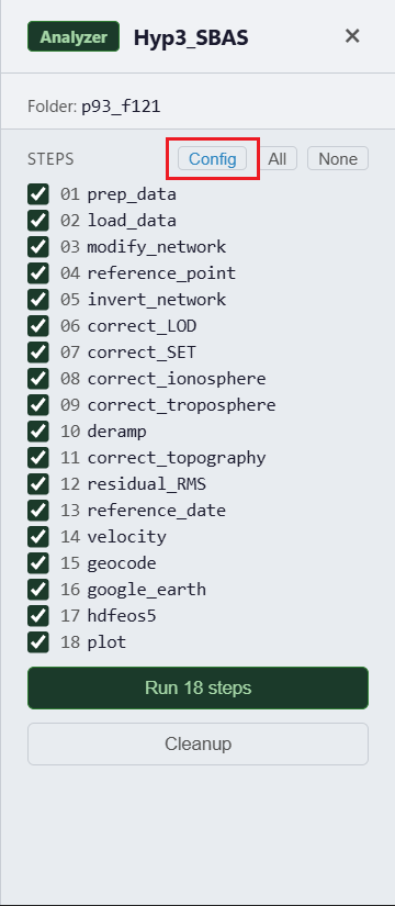
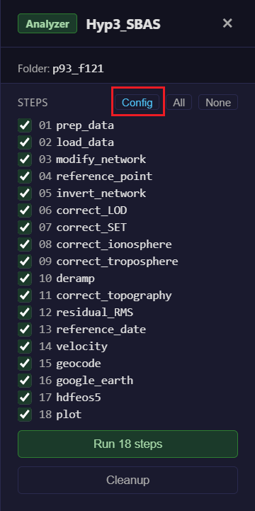
Analyzer tab.
Running Steps
Select the steps to run and click Run. Steps run sequentially and progress is shown in the log.
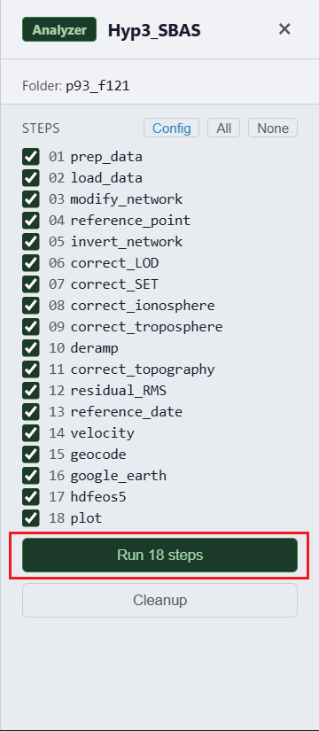
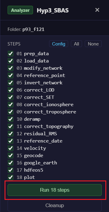
Analyzer running all steps.
Overview
After running the reference_point and quick_overview steps, an Overview button appears in the Analyzer panel. Click it to open the Overview drawer, which lets you plot MintPy diagnostic layers directly on the map.
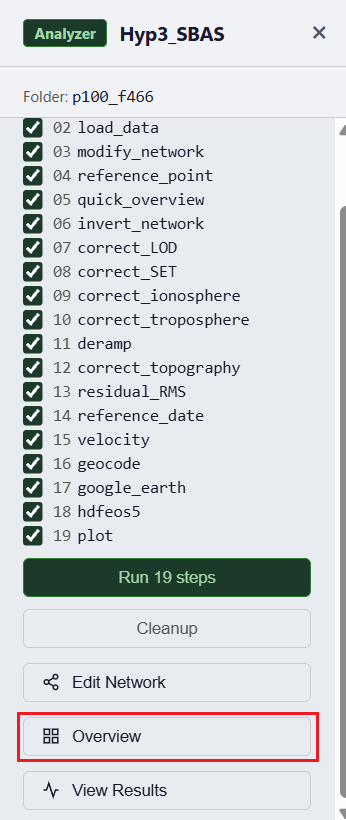
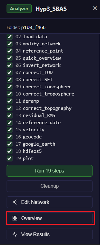
The Overview button and diagnostic layer controls in the Analyzer panel.
The Overview drawer provides four diagnostic layers:
| Button | File | What it shows |
|---|---|---|
| Avg Spatial Coherence | avgSpatialCoh.h5 |
Per-pixel average coherence across all interferograms — high values indicate reliable pixels |
| Avg Phase Velocity | avgPhaseVelocity.h5 |
Mean phase change rate — a quick sanity check for coherent deformation patterns |
| Unwrapping Error Count | numTriNonzeroIntAmbiguity.h5 |
Number of triangle closures with non-zero integer ambiguity — high counts indicate unreliable unwrapping |
| Connected Component Mask | maskConnComp.h5 |
Pixels that belong to a connected unwrapping component — isolated pixels are masked out |
Click any button to overlay that layer on the map. Click again to hide it. Hover over the map to read the pixel value in the colorbar.
Viewing Results
Once the velocity and geocode steps have completed successfully, a View Results button appears in the Analyzer panel. Click it to open the Results viewer, which overlays the computed velocity map on the main map.
Click any point on the velocity overlay to extract and display the displacement time series at that location.
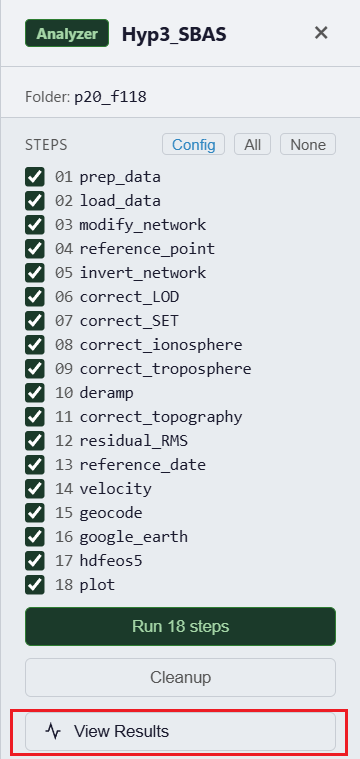
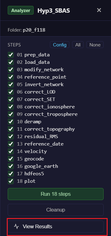
View Results button
For more details on the Results viewer, see the Results Viewer page.
Cleanup
Click Cleanup to free disk space after analysis. This removes the temporary working directories (tmp/ and clip/) and any .zip archives in the job folder that were extracted during processing. MintPy outputs, and configuration files are preserved.
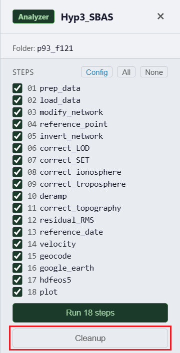
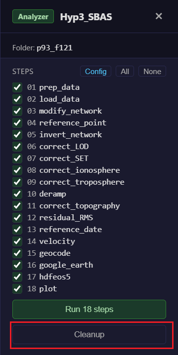
Cleanup removes intermediate HDF5 files from the working directory.