API
This section provides an overview of the complete InSAR time-series processing workflow using the Python API, guiding you through each stage of the analysis pipeline.

Modules
InSARHub is designed with three config-based main modules to cover the entire InSAR processing workflow:
You can click on each module to view detailed information later. For now, let's begin by running the program using the basic example.
Workflow
The basic workflow of InSARHub can be briefly described as:
graph
    A[Set AOI] --> B[Searching];
    B --> C[Result Filtering];
    C --> D[Interferogram];
    D --> F[Time-series Analysis];
    F --> H[Post-Processing];
    click A "#set-aoi" "Go to Set AOI section"
    click B "#searching" "Go to the Searching section"
    click C "#result-filtering" " Go to the Result Filtering section"
    click D "#interferogram"
    click F "#time-series-analysis"
    click H "#post-processing"
Set AOI
InSARHub allows you to define the AOI using a bounding box, shapefiles, or WKT:
Bounding box
Note
The AOI should be specified as [min_long, min_lat, max_long, max_lat] under CRS: EPSG:4326 (WGS84)
Shapefiles
WKT
Searching
Once the AOI is defined, you can perform searches using the Downloader.
from insarhub import Downloader
AOI = [-113.05, 37.74, -112.68, 38.00]
s1 = Downloader.create('S1_SLC', intersectsWith=AOI)
results = s1.search()
Output
Searching for SLCs....
-- A total of 991 results found.

The AOI crosses 18 stacks, you can use .summary() or .footprint() to check footprints and .filter(path_frame=(...)) to select the stack of scenes
you would like to download. If use .download() directly will create subfolders under /home/jldz9/dev/InSARHub for each stack
Result Filtering
Your AOI probably spans multiple scenes. To view the search result footprints, you can use:
This will display a footprint map of the available Sentinel-1 scenes that cover the AOI. The stack indicates the number of SAR scenes in that footprint. Because we have multiple stacks the graph will be a bit messy: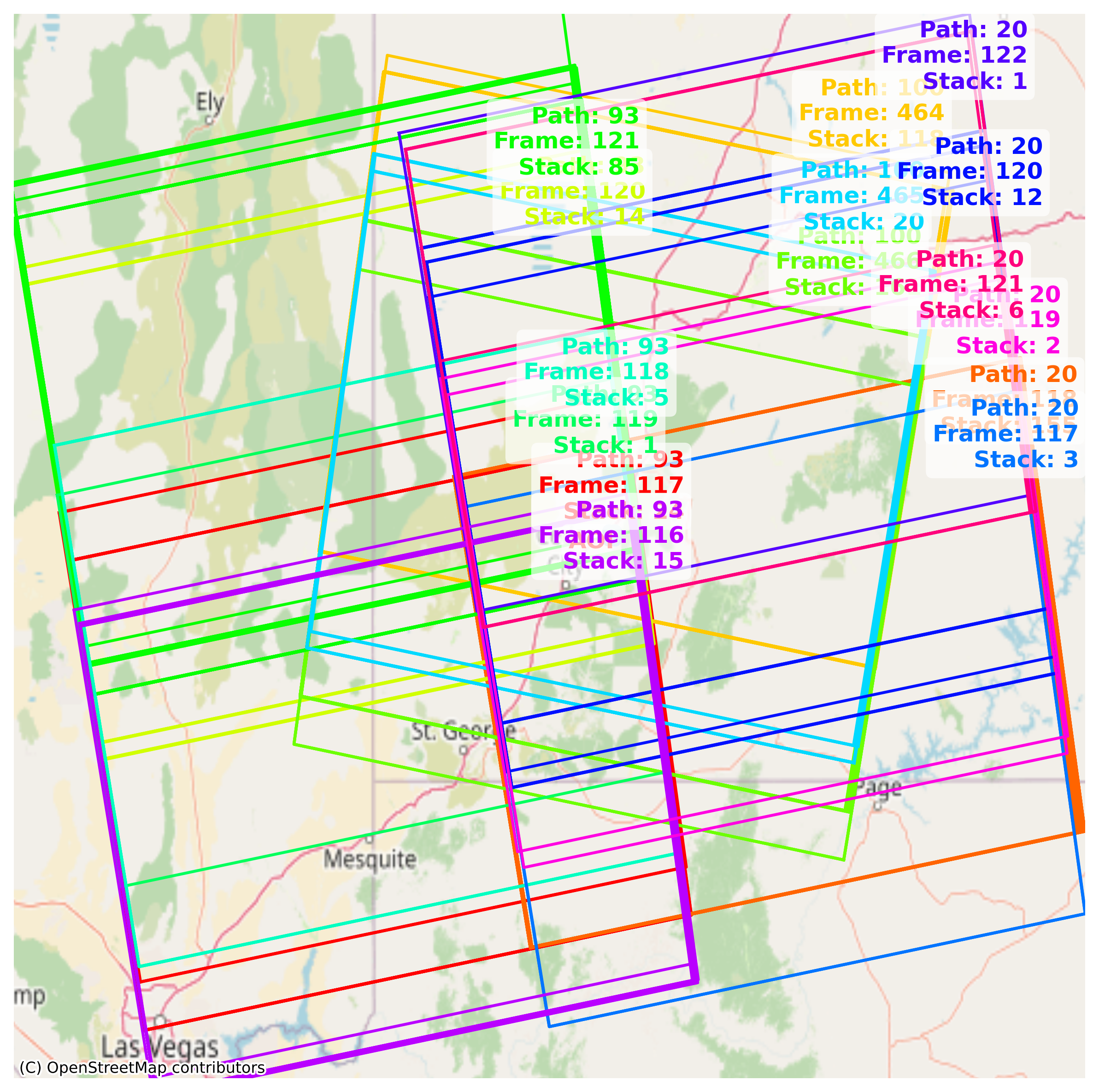
Let's check details of our SAR scene stacks and figure out which stack(s) we want to keep:
This will output the summary of available Sentinel-1 scenes that cover the AOI.Output
=== ASCENDING ORBITS (14 Stacks) ===
relativeOrbit 20 frame 117 | Count: 10 | 2015-04-05 --> 2016-11-19
relativeOrbit 20 frame 118 | Count: 156 | 2016-12-13 --> 2026-02-24
relativeOrbit 20 frame 119 | Count: 2 | 2015-03-24 --> 2015-12-25
relativeOrbit 20 frame 120 | Count: 12 | 2014-10-31 --> 2016-09-14
relativeOrbit 20 frame 121 | Count: 6 | 2015-04-05 --> 2015-08-27
relativeOrbit 20 frame 122 | Count: 4 | 2016-05-05 --> 2016-11-19
relativeOrbit 20 frame 123 | Count: 151 | 2016-12-13 --> 2026-02-24
relativeOrbit 93 frame 116 | Count: 85 | 2014-11-05 --> 2021-12-16
relativeOrbit 93 frame 117 | Count: 25 | 2015-03-29 --> 2026-03-01
relativeOrbit 93 frame 118 | Count: 5 | 2016-10-07 --> 2017-01-11
relativeOrbit 93 frame 119 | Count: 1 | 2017-02-10 --> 2017-02-10
relativeOrbit 93 frame 120 | Count: 14 | 2015-11-12 --> 2025-07-04
relativeOrbit 93 frame 121 | Count: 85 | 2014-11-05 --> 2021-12-16
relativeOrbit 93 frame 122 | Count: 22 | 2025-05-05 --> 2026-03-01

=== DESCENDING ORBITS (4 Stacks) ===
relativeOrbit 100 frame 464 | Count: 119 | 2015-11-24 --> 2026-02-23
relativeOrbit 100 frame 465 | Count: 20 | 2014-11-29 --> 2017-01-05
relativeOrbit 100 frame 466 | Count: 161 | 2017-02-22 --> 2022-07-02
relativeOrbit 100 frame 469 | Count: 119 | 2015-11-24 --> 2026-02-23
The program identified 18 potential stacks (14 ascending, 4 descending). We can narrow the dataset to the descending track Path 100, Frame 466 in year 2020 by:
Check back the footprint and summary:
would return: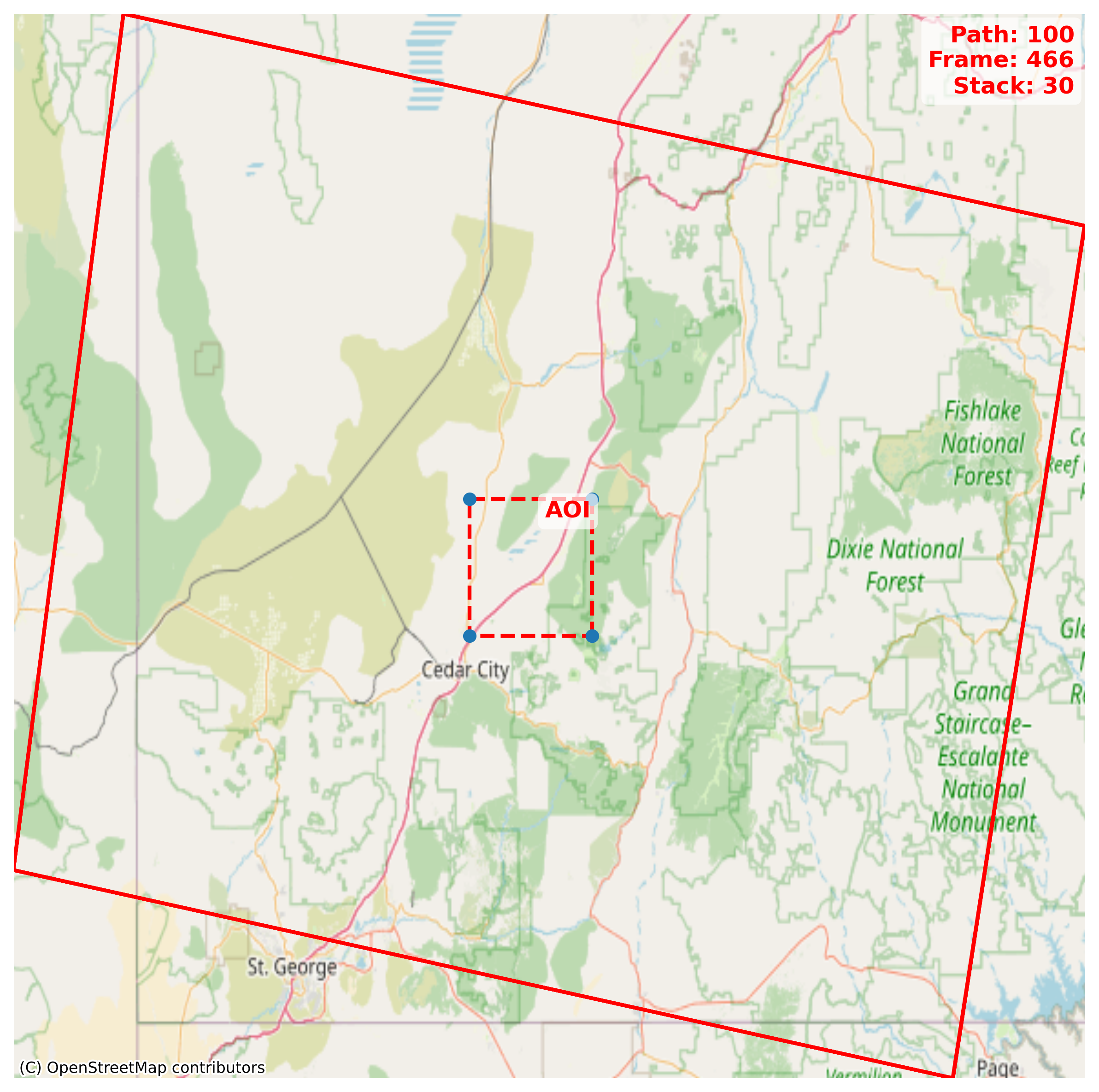
Use download to download searched SLC data
Use reset to restore original search results.
Interferogram
Select pairs
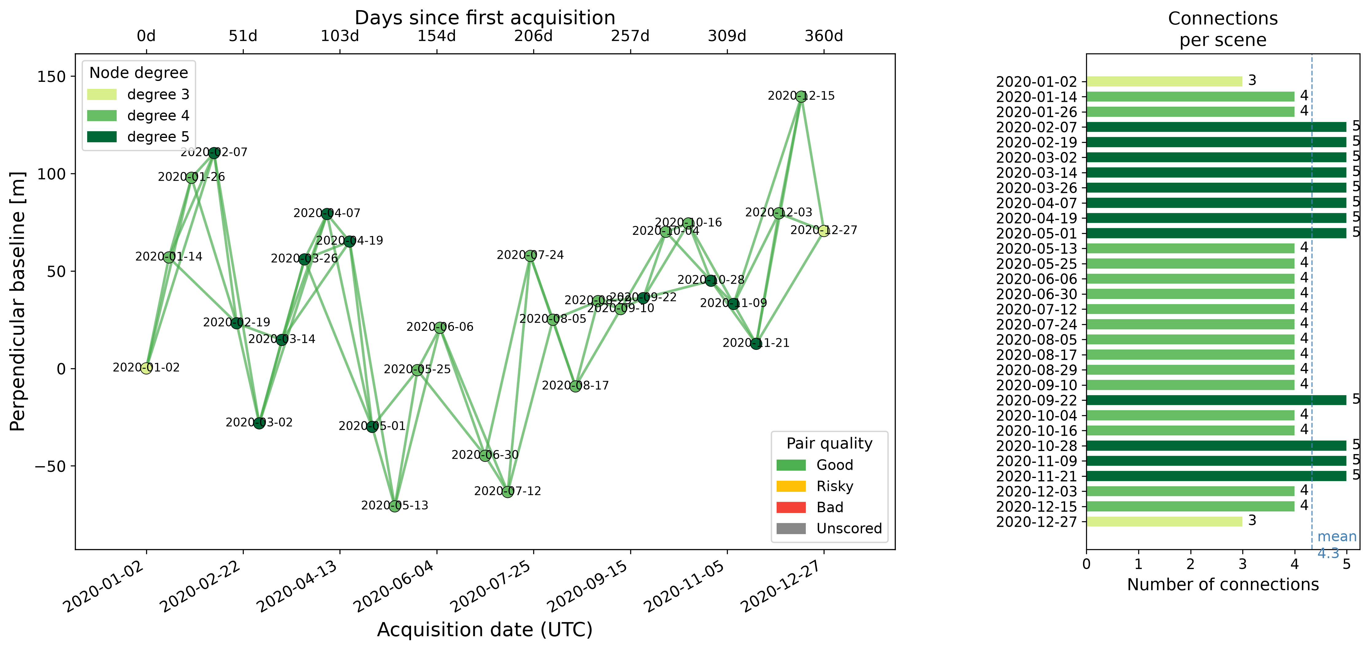
After locating SAR scene stack(s), pair selection is required to generate unwrapped interferograms for time-series analysis.
pair_stacks, B, scene_bperp, prefetch, quality_scores, quality_factors = s1.select_pairs(max_degree=5)
If the network looks healthy, continue to process interferogram:
Process Interferogram
InSARHub supports various processing methods:
Cloud-based processing via ASF HyP3 — no local ISCE2 required.
for (path, frame), pairs in pair_stacks.items():
    processor = Processor.create('Hyp3_S1', pairs=pairs, workdir=f'your/directory/p{path}_f{frame}')
    processor.submit()
    processor.save()
This generates hyp3_jobs.json in the work directory. Processing takes ~30 minutes per 100 interferograms.
To check status and download results:
Local processing using ISCE2 stackSentinel. Requires ISCE2 installed (see Installation) and SLC .SAFE files downloaded first (s1.download()).
from insarhub import Processor
from insarhub.config import ISCE2_S1_Config

for (path, frame), pairs in pair_stacks.items():
    cfg = ISCE2_S1_Config(
        workdir=f'your/directory/p{path}_f{frame}',
        bbox=[37.74, 38.00, -113.05, -112.68],   # [S, N, W, E]
        slc_dir=f'your/directory/p{path}_f{frame}/slc',
    )
    processor = Processor.create('ISCE2_S1', pairs=pairs, config=cfg)
    processor.submit()   # starts processing in the background
Dry run first
Add dry_run=True to ISCE2_S1_Config to preview run scripts without executing.
Refresh the processing status:
Output
Once all steps show SUCCEEDED, interferograms are in workdir/isce/merged/interferograms/.
Submits each step to a SLURM scheduler (sbatch) instead of running on the local machine.
from insarhub import Processor
from insarhub.config import ISCE2_S1_Config
from insarhub.processor.isce2_base import load_or_init_sbatch_options

for (path, frame), pairs in pair_stacks.items():
    cfg = ISCE2_S1_Config(
        workdir=f'your/directory/p{path}_f{frame}',
        bbox=[37.74, 38.00, -113.05, -112.68],   # [S, N, W, E]
        slc_dir=f'your/directory/p{path}_f{frame}/slc',
        hpc_mode=True,
        max_concurrent_hpc=7,
        sbatch_options_per_step=load_or_init_sbatch_options(workdir)
    )
    processor = Processor.create('ISCE2_S1', pairs=pairs, config=cfg)
    processor.submit()   # starts processing in the background
Refresh the processing status:
Runs the processing pipeline inside a prebuilt image via Docker — no local ISCE2 install needed.
from insarhub import Processor
from insarhub.config import ISCE2_S1_Config

for (path, frame), pairs in pair_stacks.items():
    cfg = ISCE2_S1_Config(
        workdir=f'your/directory/p{path}_f{frame}',
        bbox=[37.74, 38.00, -113.05, -112.68],   # [S, N, W, E]
        slc_dir=f'your/directory/p{path}_f{frame}/slc',
        container='ghcr.io/jldz9/insarhub-isce2-mintpy:0.4.0',
    )
    processor = Processor.create('ISCE2_S1', pairs=pairs, config=cfg)
    processor.submit()   # runs inside the container
Status is written to the bind-mounted workdir, so refresh() works from the host as usual:
Time-series Analysis
After generating interferograms, run MintPy SBAS time-series analysis using the matching analyzer:
The analyzer runs on the local host by default. It accepts the same container and HPC options as the processors — from either the Python API or the CLI (any *_Mintpy_SBAS analyzer):
Runs MintPy inside a prebuilt image — no local MintPy install needed (see Installation for the images).
Submits the whole analysis (prep_data → SBAS → plot) as a single sbatch job.